Attempting To Beat The Market Using RNN-Powered Sentiment Analysis
For my first research project for COMP SCI 1104, I scraped tweets mentioning several stock tickers between 2018-2019. I then isolated high volatility events for each stock ticker by daily trade volume, and tweets on that date through an RNN-based sentiment analysis model. Through an event study, I proved that sentiment polarity on twitter was an accurate proxy for determining the direction stocks would move with high statistical significance.
Methodology
Tweets from 2019 were scraped from Twitter, and daily stock close, open, high, and low price, percentage change and the trading volume of 15 selected stocks out of the 30 which served as components for the Dow Jones Industrial Average Index in 2019 was gathered from the 28th of February to the 17th of December from Yahoo Finance. Furthermore, no more than 5000 tweets are scraped per day recorded for the sake of time management (since data-scraping tends to be the most tedious aspect of such a process, and I didn’t have much time until this project was due). Each tweet was passed through a pre-trained Recurrent Neural Network (RNN) which took in the tokenized text as input and passed it through various layers of Gated Recurrent Units (GRUs), after which a 1-hot 3-vector was output representing a probability distribution of the sentiment of the tweet content being either ‘negative’, ‘neutral’, or ‘positive’.
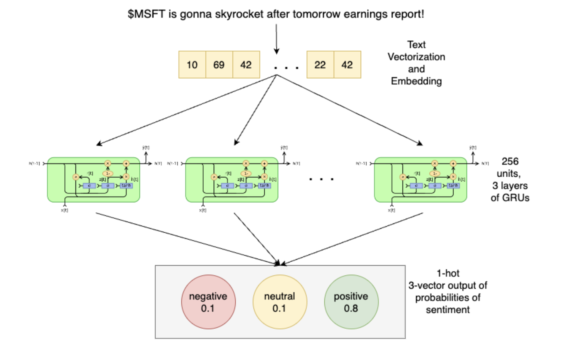 A visual representation of the RNN used to scrape through thousands of tweets for sentiment – with an input layer that leads to 3 layers containing 256 units of GRUs each, all of which eventually spit out a probability vector representing the sentiment of the input text.
All this information, alongside the daily tweet volume, the mode of sentiment, overall daily sentiment and frequency values of sentiment are dumped onto storage in the form of a JSON file by order of date, ready to be loaded for data analysis. The following highlights how some of the variables are calculated:
Let $T_d$ be the daily volume of tweets, $t_d^{-}$be the total daily negative tweets, $t_d^0$ be the total daily neutral tweets, $t_d^{+}$be the total daily positive tweets,
The sentiment polarity $P_d$ is calculated by dividing the difference between the positive and negative tweets per day by the total number of non-neutral tweets:
$$
P_d=\frac{t_d^{+}-t_d^{-}}{t_d^{+}+t_d^{-}}
$$
Analysis
During initial data exploration, the connection between sentiment and daily percentage price change wasn’t readily apparent. However, we stumbled upon a curious pattern – spikes in Twitter activity seemed to precede dramatic fluctuations in the stock price, both upwards and downwards.
Keen to understand the context of these anomalies, I explored the specific dates and the stock in question. The results were enlightening. It appeared that these surges in Twitter chatter coincided with the announcement of the company’s earnings results, aligning with the shares represented by the stock tickers.
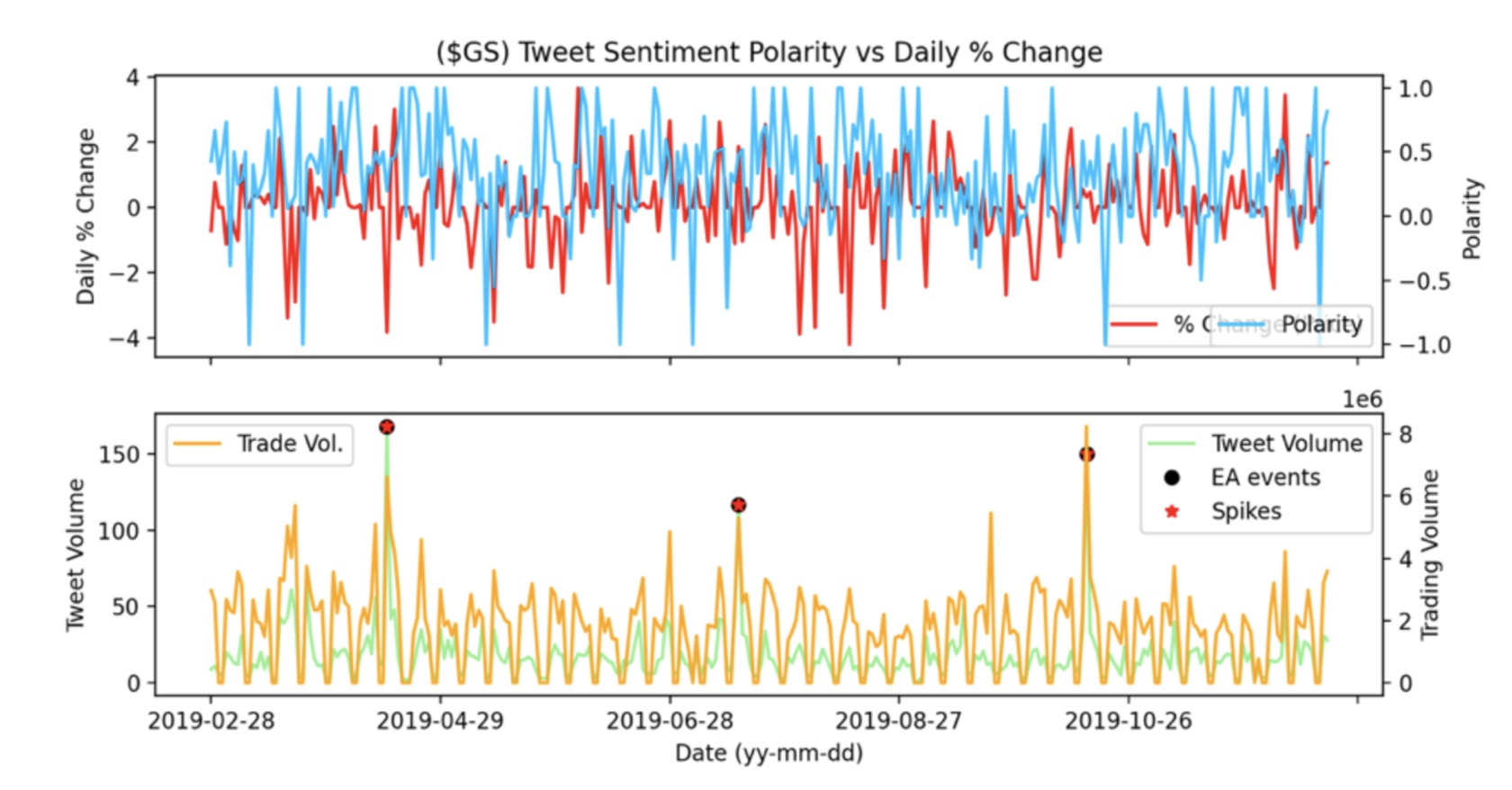 Tweet sentiment and daily price % change alongside trading and tweet volume with earnings and spike events labelled for Goldman Sach’s Stock on the NYSE. There are gaps in trade volume and price change data on holidays and weekends when the stock exchanges are closed. Notice, how tweeting and trading volume spikes during/the day after an earnings announcement, and in some cases, also appear to cause large movements in the GS ’s price.
This finding hinted at an intriguing prospect: Twitter volume might be a promising predictor of stock movements. To validate this hypothesis, I took a more rigorous approach. I computed the Pearson correlation coefficients and executed Granger-causality tests (with a 3-day lag) between the previously mentioned variables. My analysis included absolute percentage price change, rather than just the percentage price change, given that volume cannot fall below zero.
Based on my observations thus far, it seemed only logical to examine further whether these spike events in Twitter activity do indeed influence stock prices.
Event Study
In this exploration, we will employ an event study method – a commonly used analytical approach in financial econometrics (as defined by John Y. Campbell, 1996). This technique investigates the ‘abnormal returns’ of an asset during specific external events.
To kick-start the process, we need to pinpoint a series of unusual events for each stock ticker. The polarity of these events also needs to be identified, as it would hint towards the event’s positive or negative influence on the stock’s price. Additionally, a rolling event window and a market model are necessary to measure the ‘abnormal returns’ following these unusual spikes in Twitter activity.
Now, ‘normal returns’ refer to what the stock would have gained if these extraordinary events hadn’t transpired. To calculate the abnormal returns, we use the following formula:
\[AR_{i,d}=R_{i,d}-E\left[R_{i,d}\right]\]Here, $AR_{i,d},\ R_{i,d},$ and $E\left[R_{i,d}\right]$ denote the abnormal return, actual return, and normal return respectively. I assume a constant-mean-return model to estimate normal returns, which implies that a security’s average return remains stable throughout.
To compute the mean return E\left[R_{i,d}\right] for each stock ticker on a given date, I calculated their average percentage return throughout 2018, and also consider the standard deviation and variance of each stock’s respective return.
Armed with these parameters, I can now calculate the abnormal returns. I start with the null hypothesis ($H_0$) that Twitter spike events don’t affect the resulting abnormal returns. Campbell (1996) showed that under $H_0$, these returns follow a normal distribution.
We then perform Twitter peak detection by calculating the median volume in a 14-day window. Any activity exceeding 3 standard deviations of this median volume is considered a ‘spike’ event. Each spike is assigned a polarity based on the sentiment polarity, indicating whether it would positively or negatively impact the stock’s price.
Sentiment polarity ranges from -1 to 1, with thresholds defined as follows for negative, neutral, and positive events:
When $P_d<0.2$, the event is classified as negative
When $P_d\in\left[0.2,0.6\right]$, the event is classified as neutral
When $P_d>0.6$, the event is classified as positive
The cumulative abnormal return (CAR) of a stock is calculated as the actual return minus the normal return over a chosen event window of -5 to 10 days from the detected spike event.
These values must be aggregated to draw meaningful conclusions from the data. Aggregation is performed across all selected stocks and over time, yielding at a certain date:
\[\overline{AR_\tau}=\frac{1}{N}\sum_{i=1}^{N}{AR_{i,\tau}}\]The CAR from \tau_1 to \tau_2 is the sum of the abnormal returns:
\[CAR\left(\tau_1,\tau_2\right)=\sum_{\tau=\tau_1}^{\tau_2}\overline{AR_\tau}\]The variance of CAR is calculated as follows:
\[var\left(CAR\left(\tau_1,\tau_2\right)\right)=\frac{1}{N^2}\sum_{i=1}^{N}{\left(\tau_2-\tau_1\right)\sigma_{\epsilon_i}^2\ }\]Where $N$ is the total number of events. Finally, we arrive at the test statistic \hat{\theta}, which helps us gauge the impact of an event on the abnormal returns of all tested stocks:
\[\frac{CAR\left(\tau_1,\tau_2\right)}{\sqrt{var\left(CAR\left(\tau_1,\tau_2\right)\right)}}= \hat{\theta} \sim N\left(0,1\right)\]In the above equation, $\tau$ is a timestamp within the event window, with $\tau_1$ as the initial timestamp and $\tau_2$ as the final one.
Results
After running calculations for Pearson’s coefficient for tweet volume vs. abs. return % and polarity and return %, along with granger-cause tests as well, it was apparent that there was little to no forecasting power available for price movements given tweet polarity. Yet, there was a moderate correlation between tweet volume and absolute return % (with values p-values ranging between ~0.4-~0.7). Regardless, the null hypothesis, that tweet sentiment polarity does not affect price movement direction, must be accepted.
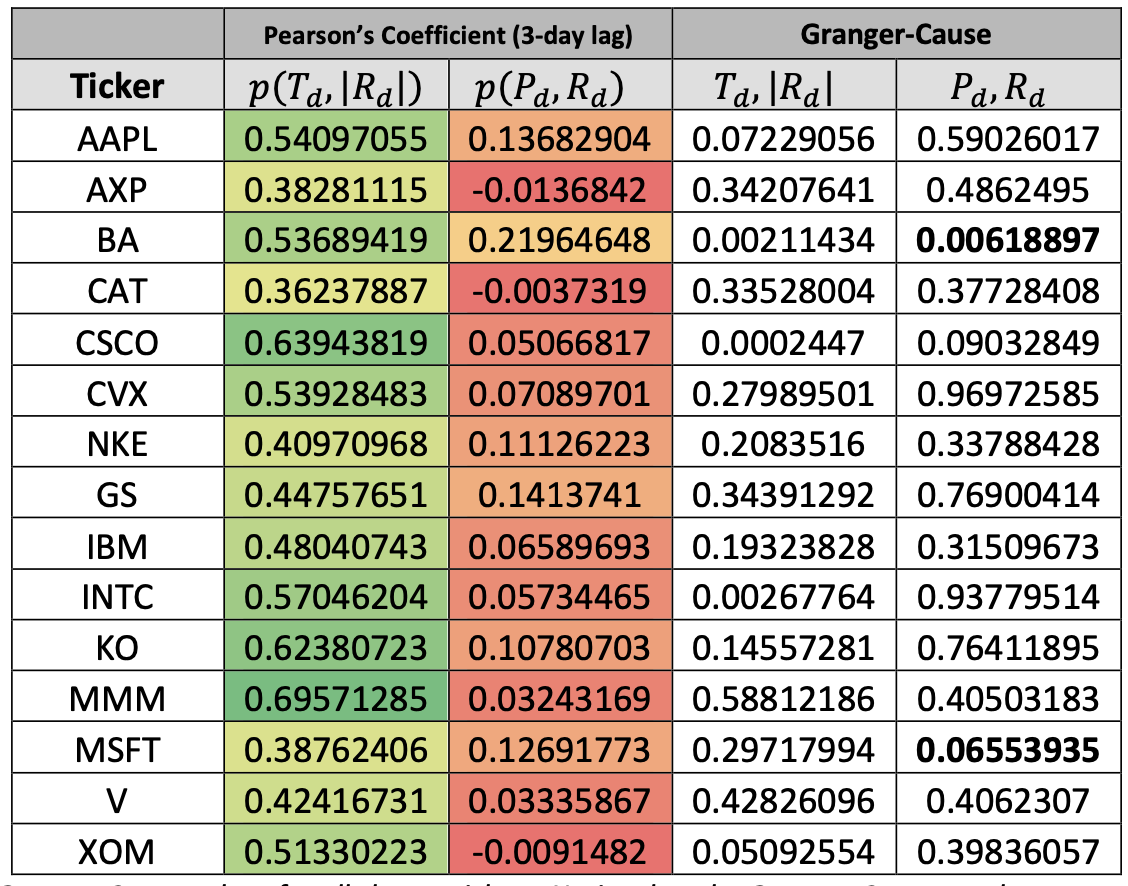 Pearson’s and Granger Cause values for all chosen tickers. Notice that the Granger-Cause test between polarity and % returns only passes (<0.05) for only 2 of the stocks, yet the p-values indicate a moderate correlation between tweet volume and absolute return % given a 3- day lag period
However, even though polarity may not always correlate with price movement, it appears it can be used as a proxy for predicting price prediction during tweet volume spike events. The following visualises the impact of such spike events on the CAR (%) aggregated from all 15 stocks:
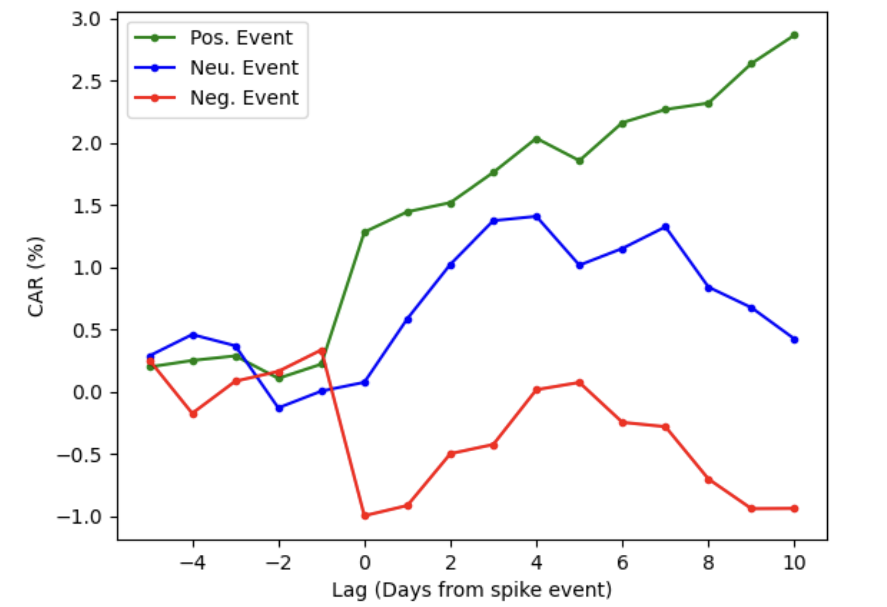
Armed with our data, we’re now set to compute the test statistic to examine the statistical significance of tweet spikes. Notably, the variance of the Cumulative Abnormal Return (CAR) stands around 0.025%, with abnormal returns of roughly 1.28% for positive events and -1% for negative events. This crunches down to a test statistic of around 8.01 for positive events and -6.32 for negative ones, effectively overturning the null hypothesis - tweet spikes indeed wield significant sway over stock returns.
Interestingly, the sentiment (or polarity) of tweets about a particular stock seems to hint at the stock’s future trajectory. In essence, if the test statistic returns values above 1 for positive events (or below -1 for negative ones), we can anticipate a similar movement in stock returns even days post-event. However, it’s intriguing to note that neutral events often lead to positive returns, hinting that our categorization of polarity thresholds could use some tweaking.